How to Read a Welchs Two Sample T-test in R

Welch T-Exam

The independent samples t-test comes in ii dissimilar forms:

the standard Student'due south t-test, which assumes that the variance of the two groups are equal.
the Welch'south t-test, which is less restrictive compared to the original Student'south test. This is the examination where you do not presume that the variance is the same in the two groups, which results in the partial degrees of freedom.

Note that, the Welch t-examination is considered as the safer one. Usually, the results of the classical student'due south t-exam and the Welch t-exam are very like unless both the group sizes and the standard deviations are very different.

This article describes the Welch t-test, which is an accommodation of the Student'southward t-test for comparison the means of 2 contained groups, in the state of affairs where the homogeneity of variance assumption is not met. The Welch t-test is also referred every bit: Welch'due south t-test, Welchs t-examination, t-test unequal variance, t-exam assuming diff variances or carve up variance t-test

In this article, you volition acquire:

Welch t-test formula and assumptions
How to compute, interpret and report the Welch t-examination in R.
How to cheque the Welch t-test assumptions

Contents:

Prerequisites
Research questions
Statistical hypotheses
Formula
Assumptions and preleminary tests
Computing the test in R
- Demo data
- Summary statistics
- Visualization
- Computation
- Cohen's d for Welch t-test
Report
Summary

Related Volume

Practical Statistics in R 2 - Comparing Groups: Numerical Variables

Prerequisites

Brand sure you take installed the following R packages:

tidyverse for data manipulation and visualization
ggpubr for creating hands publication set plots
rstatix provides piping-friendly R functions for easy statistical analyses.
datarium: contains required information sets for this chapter.

Start by loading the following required packages:

                  library(tidyverse) library(ggpubr) library(rstatix)

Research questions

A typical research questions is: whether the mean of group A (\(m_A\)) is equal to the hateful of group B (\(m_B\))?

Statistical hypotheses

Cypher hypothesis (Ho): the ii group ways are identical (\(m_A = m_B\))
Alternative hypothesis (Ha): the two group means are different (\(m_A \ne m_B\))

Formula

The Welch t-statistic is calculated as follow :

\[
t = \frac{m_A - m_B}{\sqrt{ \frac{S_A^two}{n_A} + \frac{S_B^2}{n_B} }}
\]

where, \(S_A\) and \(S_B\) are the standard difference of the the two groups A and B, respectively.

Unlike the classic Student's t-test, the Welch t-examination formula involves the variance of each of the two groups (\(S_A^two\) and \(S_B^2\)) existence compared. In other words, information technology does not use the pooled variance\(S\).

The degrees of freedom of Welch t-test is estimated as follow :

\[
df = (\frac{S_A^2}{n_A}+ \frac{S_B^2}{n_B})^2 / (\frac{S_A^iv}{n_A^2(n_A-1)} + \frac{S_B^iv}{n_B^2(n_B-1)} )
\]

A p-value can be computed for the corresponding absolute value of t-statistic (|t|).

If the p-value is inferior or equal to the significance level 0.05, nosotros tin can turn down the null hypothesis and accept the alternative hypothesis. In other words, nosotros tin conclude that the mean values of group A and B are significantly different.

Assumptions and preleminary tests

The Welch t-test assumes the following characteristics about the data:

Independence of the observations. Each subject should belong to only one group.
No significant outliers in the ii groups
Normality. the data for each group should be approximately unremarkably distributed.

Click to cheque the Student t-exam assumptions.

Calculating the exam in R

Demo information

Demo dataset: genderweight [in datarium packet] containing the weight of 40 individuals (20 women and 20 men).

Load the data and show some random rows by groups:

                    # Load the data data("genderweight", package = "datarium") # Bear witness a sample of the information by grouping prepare.seed(123) genderweight %>% sample_n_by(grouping, size = 2)

                    ## # A tibble: 4 x iii ##   id    group weight ##   <fct> <fct>  <dbl> ## one 6     F       65.0 ## 2 15    F       65.9 ## 3 29    M       88.9 ## four 37    M       77.0

Summary statistics

Compute some summary statistics past groups: hateful and sd (standard divergence)

                    genderweight %>%   group_by(group) %>%   get_summary_stats(weight, type = "mean_sd")

                    ## # A tibble: 2 x 5 ##   group variable     n  mean    sd ##   <fct> <chr>    <dbl> <dbl> <dbl> ## 1 F     weight      twenty  63.5  two.03 ## two M     weight      20  85.8  four.35

Visualization

Visualize the information using box plots. Plot weight by groups.

                    bxp <- ggboxplot(   genderweight, x = "group", y = "weight",    ylab = "Weight", xlab = "Groups", add = "jitter"   ) bxp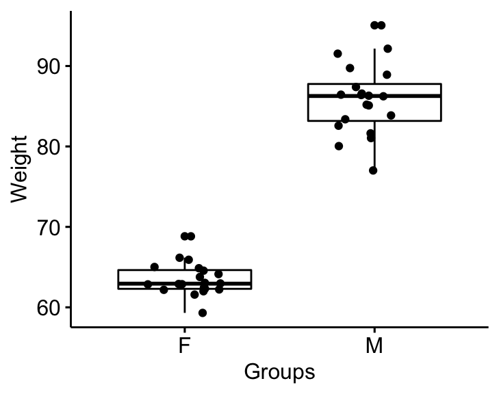

Computation

Nosotros'll apply the pipage-friendly t_test() function [rstatix parcel], a wrapper effectually the R base function t.test().

Recall that, past default, R computes the Welch t-test, which is the safer ane. This is the examination where yous do not assume that the variance is the same in the two groups, which results in the fractional degrees of freedom. If you want to assume the equality of variances (Student t-test), specify the option var.equal = True.

                    stat.test <- genderweight %>%   t_test(weight ~ group) %>%   add_significance() stat.test

                    ## # A tibble: 1 10 9 ##   .y.    group1 group2    n1    n2 statistic    df        p p.signif ##   <chr>  <chr>  <chr>  <int> <int>     <dbl> <dbl>    <dbl> <chr>    ## 1 weight F      G         20    xx     -20.viii  26.ix 4.30e-18 ****

The results to a higher place show the following components:

.y.: the y variable used in the test.
group1,group2: the compared groups in the pairwise tests.
statistic: Test statistic used to compute the p-value.
df: degrees of liberty.
p: p-value.

Annotation that, you can obtain a detailed upshot by specifying the selection detailed = TRUE.

Cohen's d for Welch t-test

The effect size can be computed by dividing the mean departure between the groups by the "averaged" standard deviation.

Cohen's d formula:

d = (mean1 - mean2)/sqrt((var1 + var2)/2), where:

mean1 and mean2 are the means of each group, respectively
var1 and var2 are the variance of the two groups.

Adding:

                    genderweight %>% cohens_d(weight ~ group, var.equal = FALSE)

                    ## # A tibble: 1 ten 7 ##   .y.    group1 group2 effsize    n1    n2 magnitude ## * <chr>  <chr>  <chr>    <dbl> <int> <int> <ord>     ## ane weight F      Yard        -6.57    20    xx big

Written report

We could study the result as follow:

The hateful weight in female group was 63.five (SD = two.03), whereas the mean in male person group was 85.8 (SD = 4.iii). A Welch two-samples t-test showed that the difference was statistically significant, t(26.9) = -xx.viii, p < 0.0001, d = 6.57; where, t(26.nine) is shorthand annotation for a Welch t-statistic that has 26.9 degrees of freedom.

                  stat.test <- stat.test %>% add_xy_position(x = "group") bxp +    stat_pvalue_manual(stat.test, tip.length = 0) +   labs(subtitle = get_test_label(stat.test, detailed = Truthful))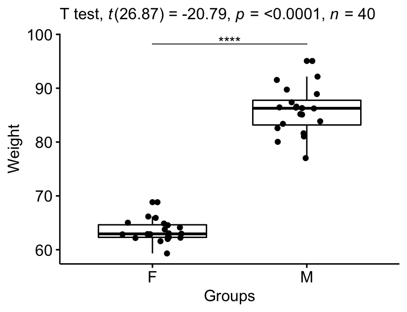

Summary

This article describes the formula and the basics of the Welch t-test. Examples of R codes are provided for computing the test and the effect size, interpreting and reporting the results.

Recommended for you

This section contains best data science and cocky-development resources to aid you on your path.

Version: Français

Back to T-Test Essentials: Definition, Formula and Adding

freemanandii1971.blogspot.com

Source: https://www.datanovia.com/en/lessons/types-of-t-test/unpaired-t-test/welch-t-test/